Thesis Chapters
Click on a chapter to explore its contents
Introduction
From resolution limits to AI-powered reconstruction
Modern science is inconceivable without interdisciplinary research. This chapter introduces the three software projects developed during this thesis: LineProfiler for evaluating filamentous structures, Automated Simple Elastix for validating expansion microscopy, and ReCSAI for reconstructing non-linear point spread functions using AI.
Key Figures
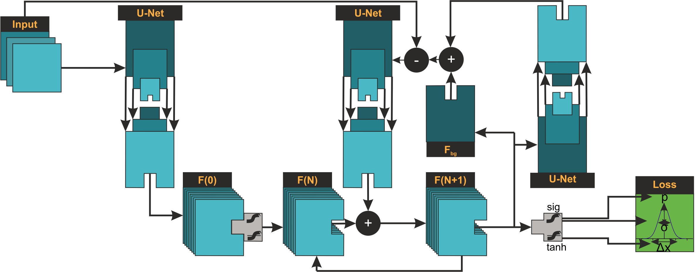
ReCSAI architecture: Recursive algorithm unrolling integrates Compressed Sensing directly into the neural network, enabling iterative refinement between feature and image space for superior reconstruction of non-linear PSFs.
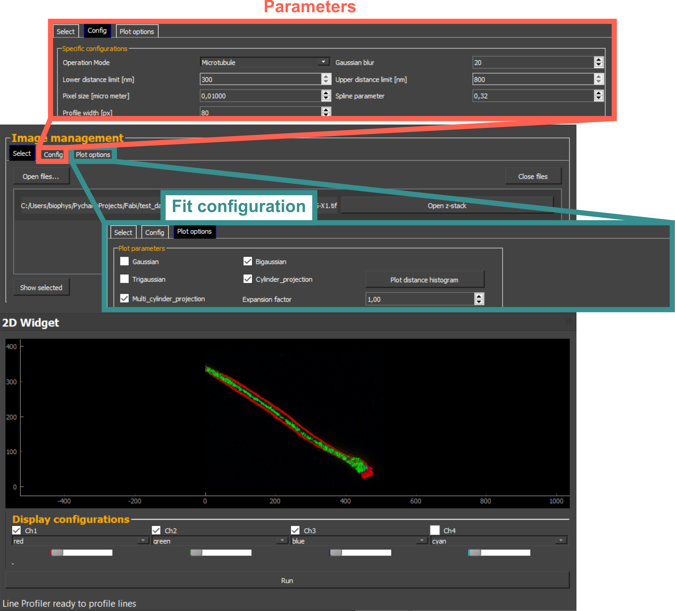
LineProfiler interface: Objective tool for evaluating filamentous structures. Instead of manually selecting regions, the software automatically collects profiles from the entire image, preventing biased sampling.
Theory of Super-Resolution Microscopy
Breaking the diffraction limit
Why is classical light microscopy limited? This chapter explains the Abbe/Rayleigh resolution limit, fluorescence physics (Frank-Condon principle, Jablonski diagrams), microscopy modalities (TIRF, confocal), fluorescence lifetime imaging (FLIM), and noise sources in detectors.
Key Figures
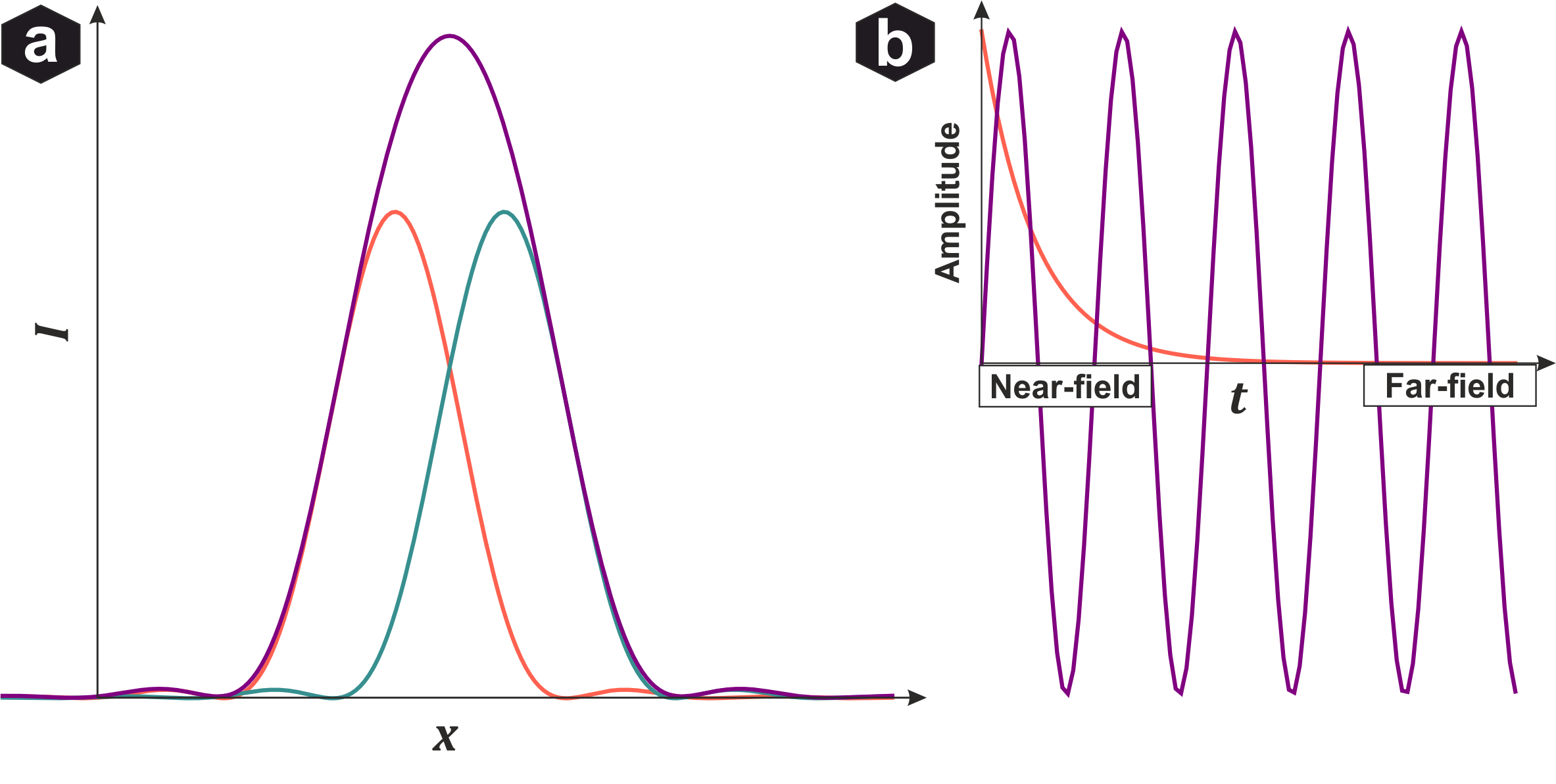
Resolution limit: (a) Rayleigh criterion - if the PSF maximum of one emitter overlaps more than the first minimum of another, they cannot be distinguished and appear as one. (b) Propagation into far field - larger spatial frequencies decay exponentially and are lost.
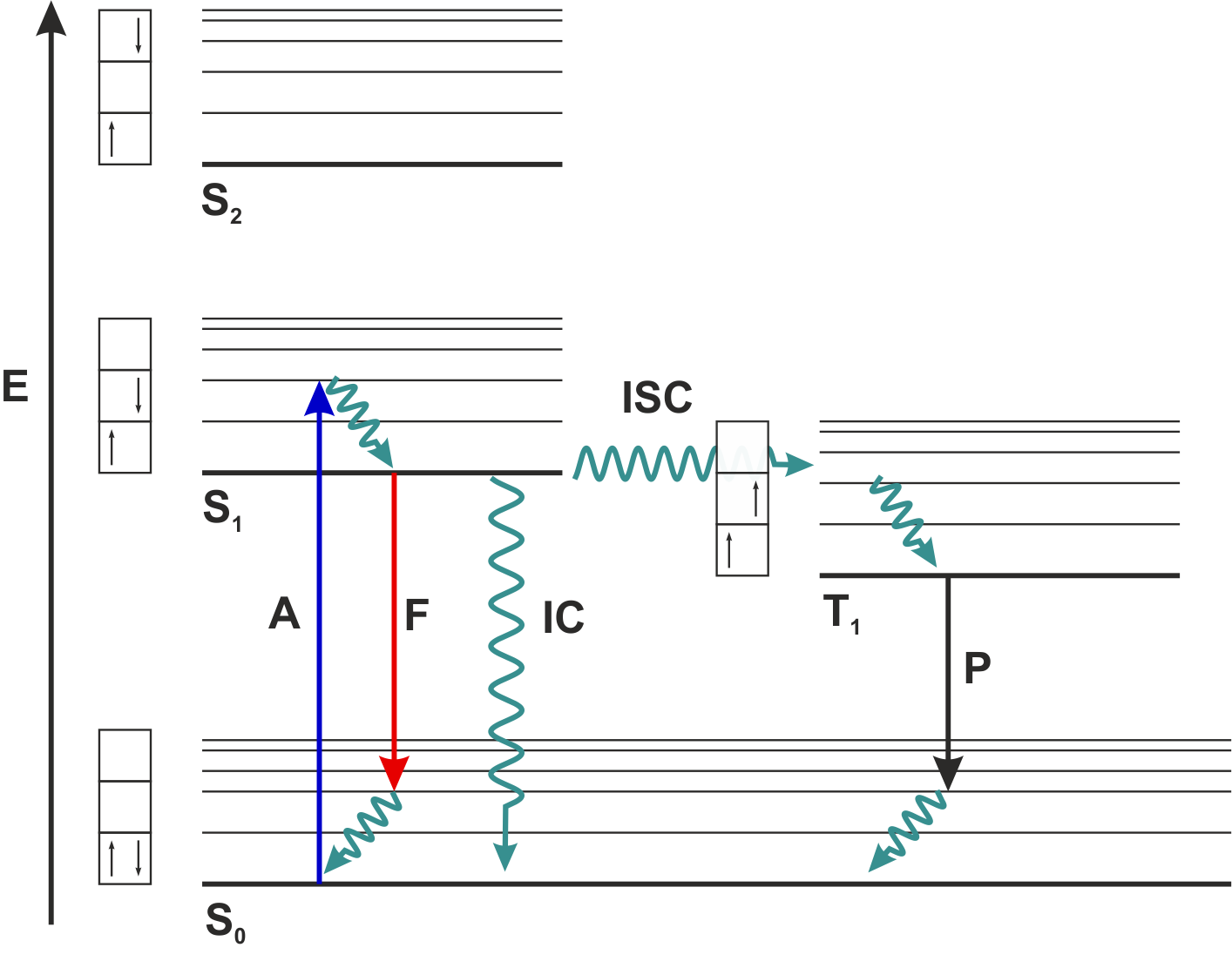
Jablonski diagram: Electrons in singlet ground-state S₀ are excited to S₁ by photon absorption. Relaxation occurs via Fluorescence (F) or Internal Conversion (IC). Small probability exists for Inter-System Crossing (ISC) to long-lived triplet state T₁.
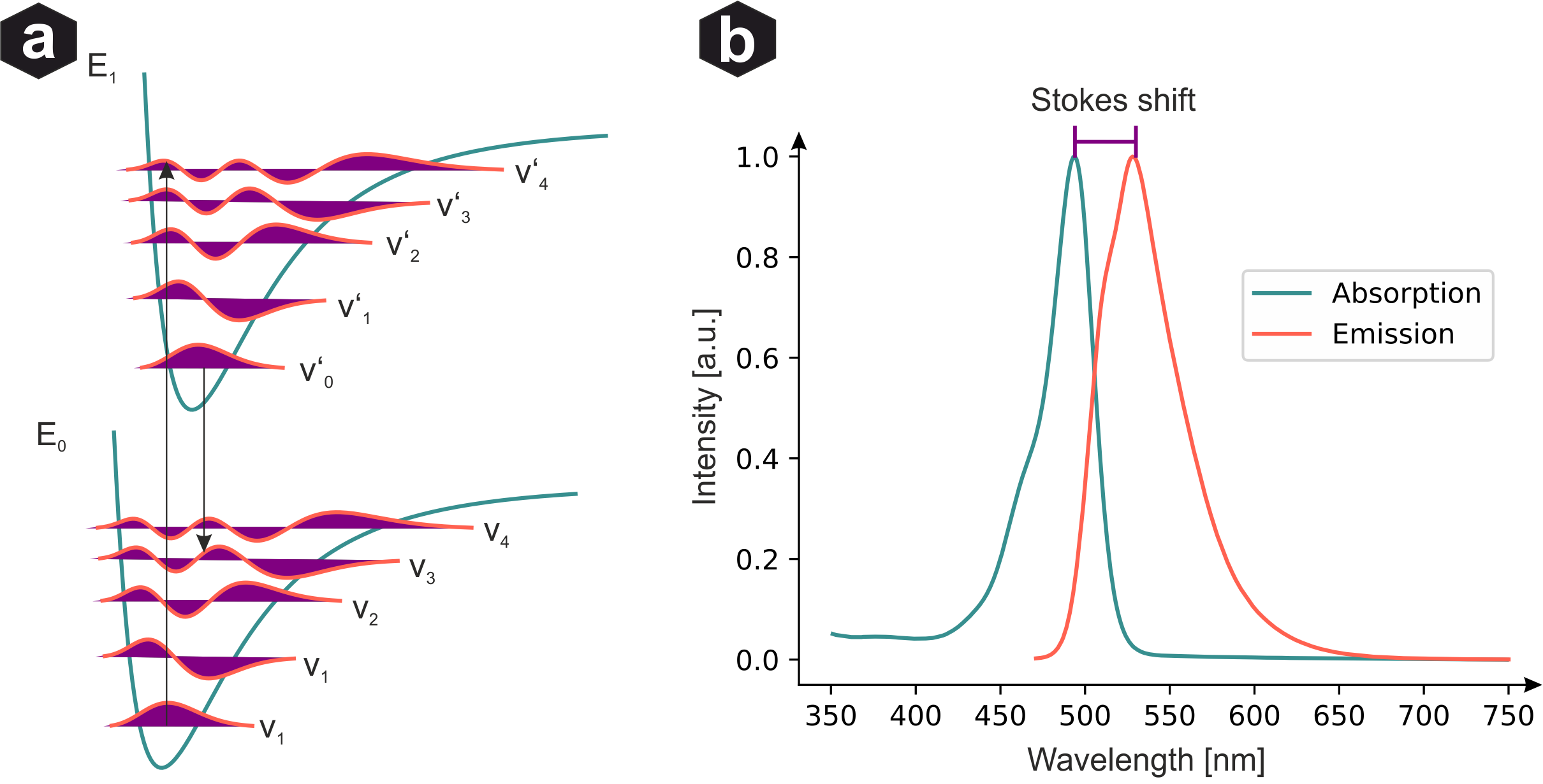
Frank-Condon principle: (a) Ground E₀ and excited E₁ states with vibrational levels. Transition probabilities given by wavefunction overlap. Absorption excites to higher vibrational level, then rapid non-radiative decay before emission. (b) Measured emission/absorption spectra showing Stokes shift.
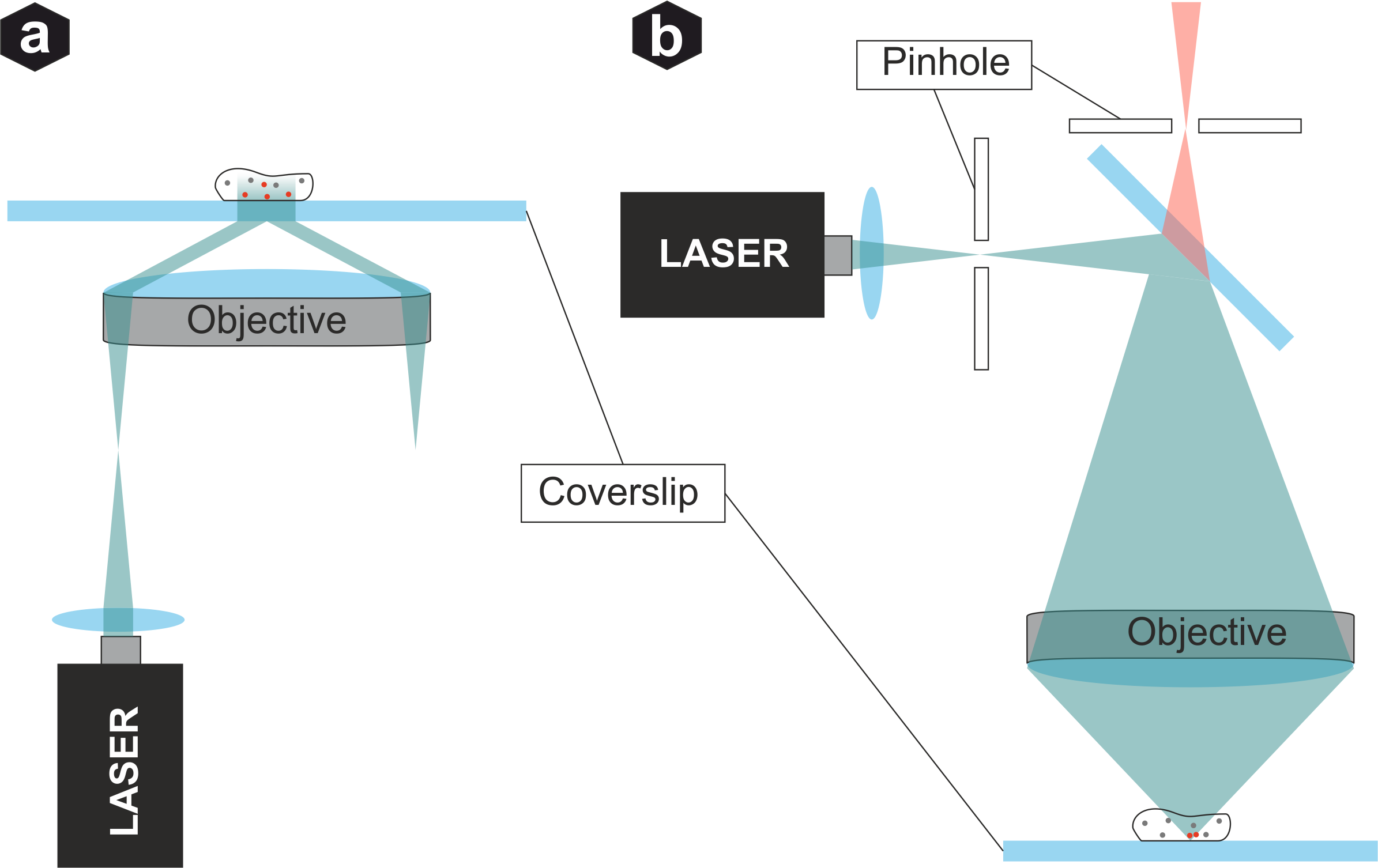
Microscopy modalities: (a) TIRF - excitation beam totally reflected at coverslip, creating evanescent wave that only excites emitters very close to surface. (b) Confocal - pinhole filters out-of-focus signals, enabling 3D resolution and enhanced contrast.
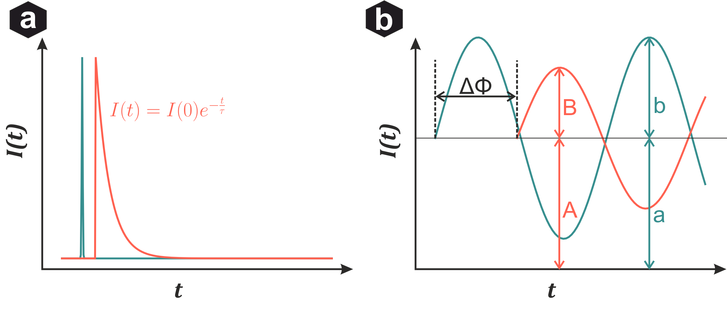
Fluorescence-Lifetime Imaging: (a) Time-domain - short laser pulse excitation, lifetime from exponential intensity decay. (b) Frequency-domain - modulated excitation intensity, lifetime calculated from phase shift and amplitude modulation.
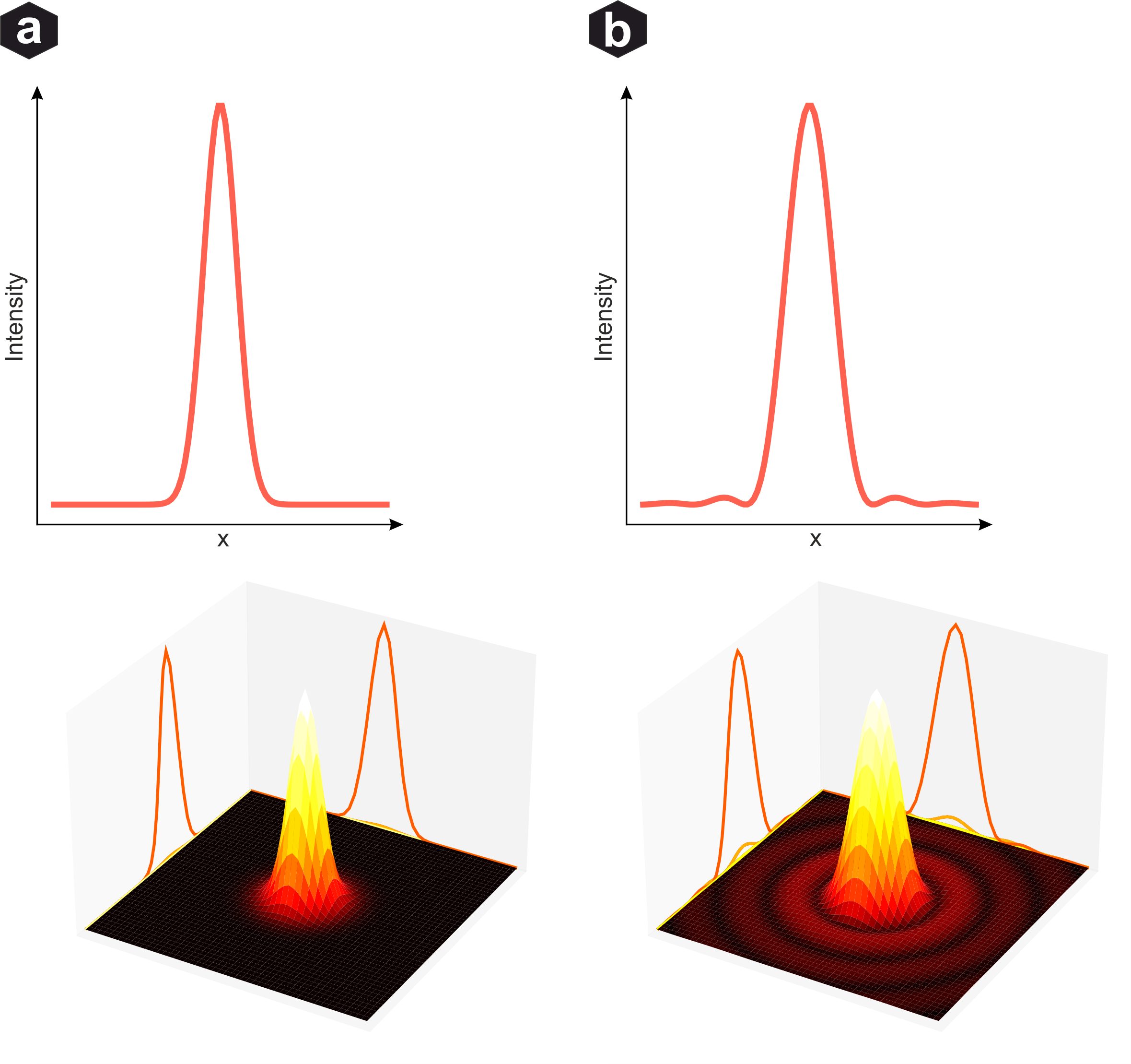
Gaussian distribution vs Airy disc: Despite the Airy disc being theoretically more accurate, the Gaussian approximation performs well for reconstruction since its mean equals the center of mass. Side maxima often reside below noise level.
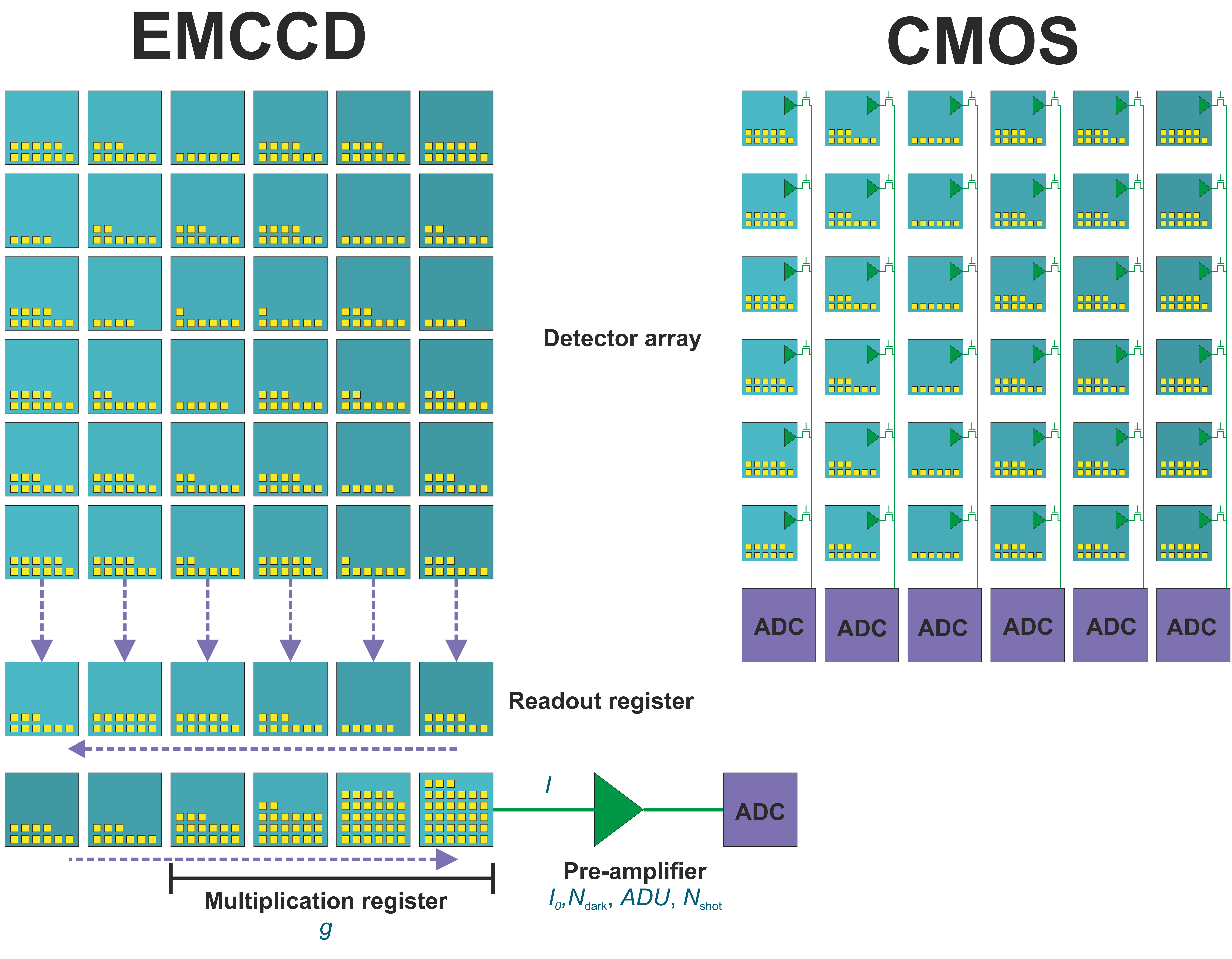
EMCCD and CMOS detectors: EMCCD collects electrons in photodiode, shifts through multiplication register for amplification, then converts to digital. CMOS has per-pixel transistors with microlenses to focus light on reduced photoactive area.
Sections
Signal Processing & Neural Networks
From Fourier transforms to deep learning
The algorithmic foundations: Fourier transforms, convolution, wavelet analysis, and the evolution from classical signal processing to modern deep learning. Covers neural network architectures including dense layers, CNNs, U-Net, ResNet, and training optimization.
Key Figures
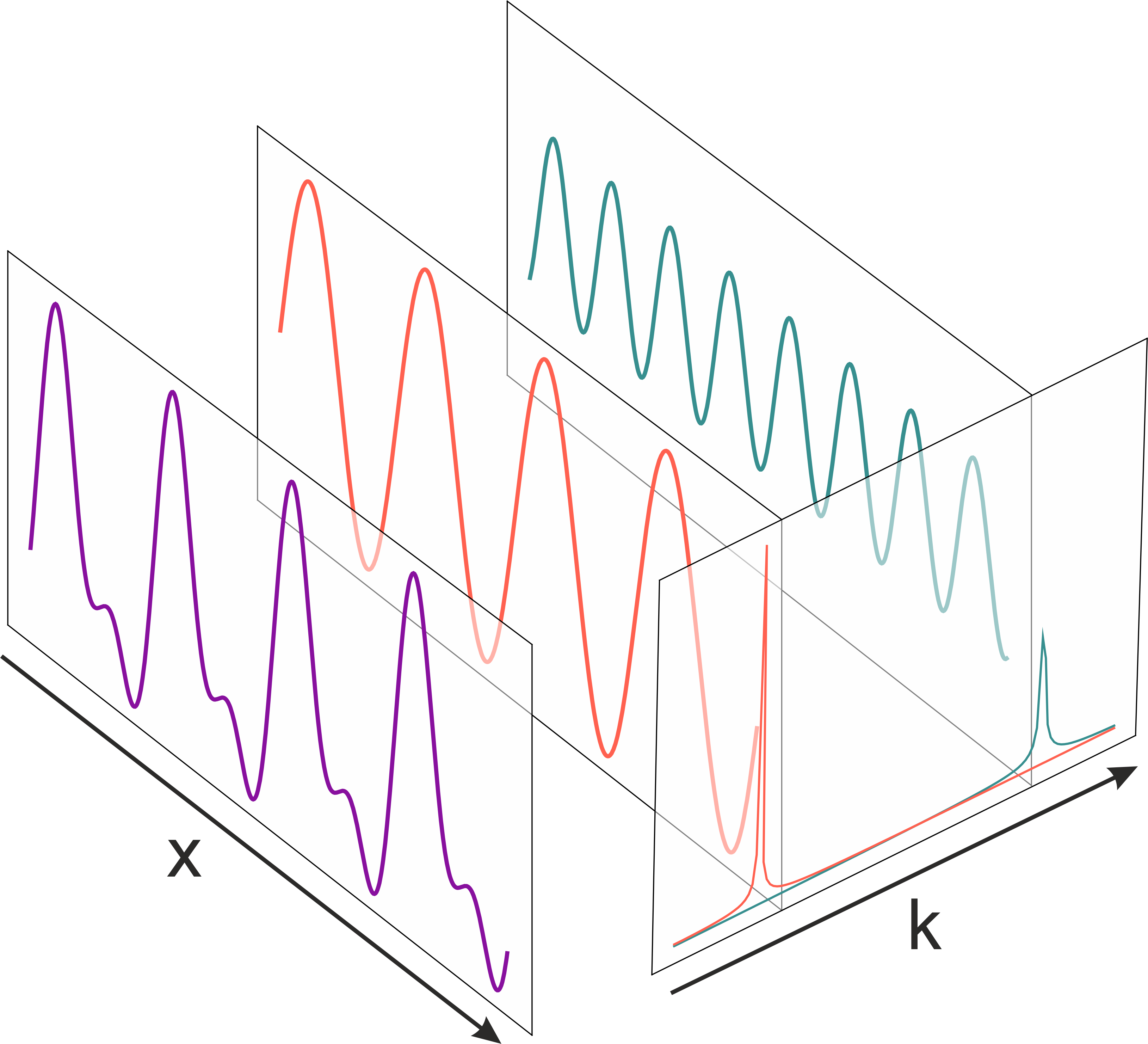
The Fourier transform decomposes a signal of superimposed sine waves into complex numbers. The real part contains amplitude information, the imaginary part contains phase. Superimposing signals with same frequency but different phases/amplitudes yields new signal with identical frequency.
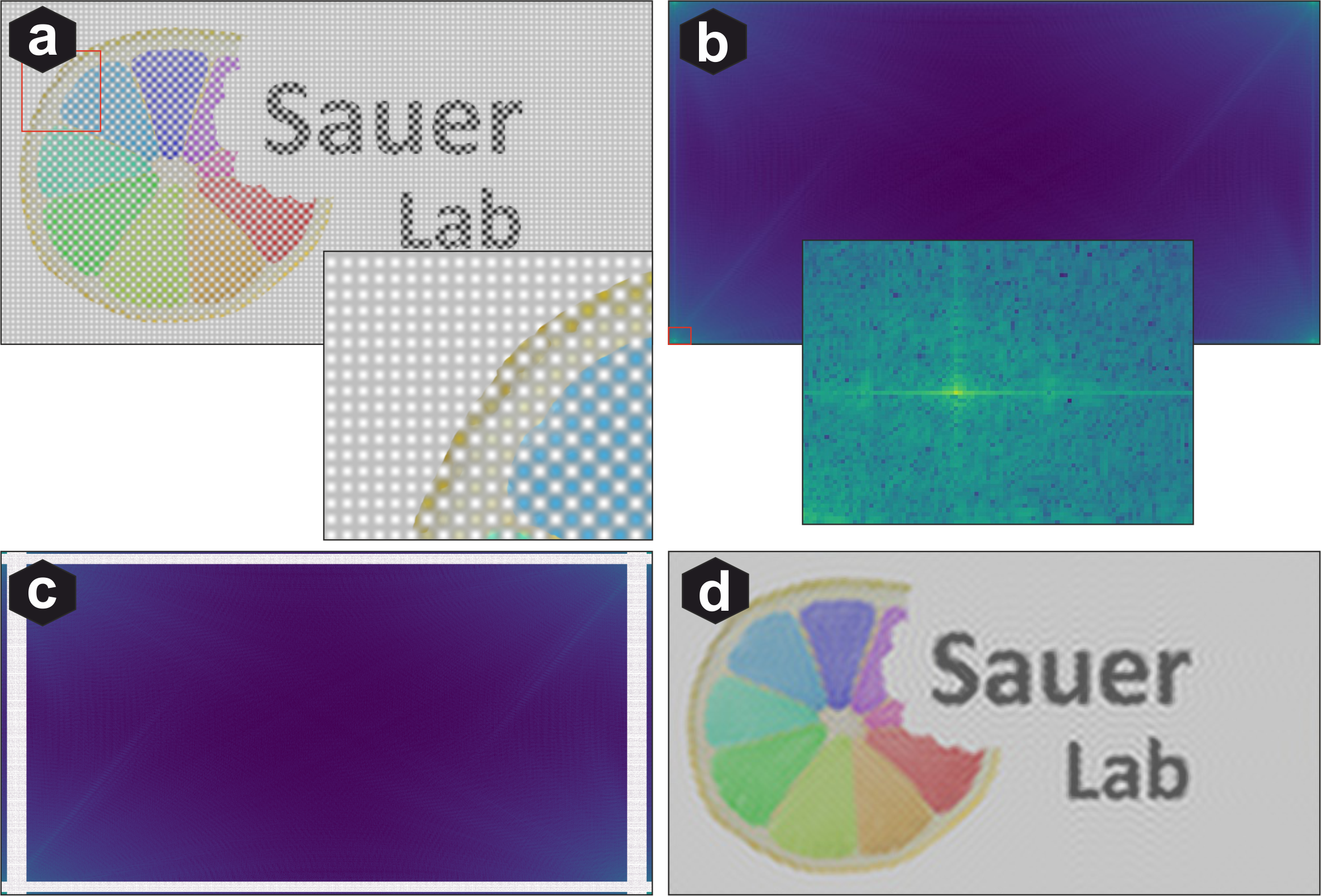
Fourier transform of images: (a) Image with pattern noise. (b) Patterns appear as peaks at specific frequencies in Fourier space. (c) Removing those frequency bands eliminates the patterns. (d) Removing broader bands also degrades overall image quality.
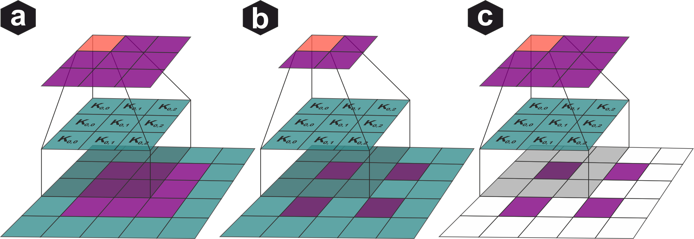
Discrete convolution: Each output pixel is computed by multiplying input values with kernel weights and summing. Common linear filters shown: Gaussian (smoothing), Prewitt (edge detection), Laplacian (second derivative) with their frequency characteristics.
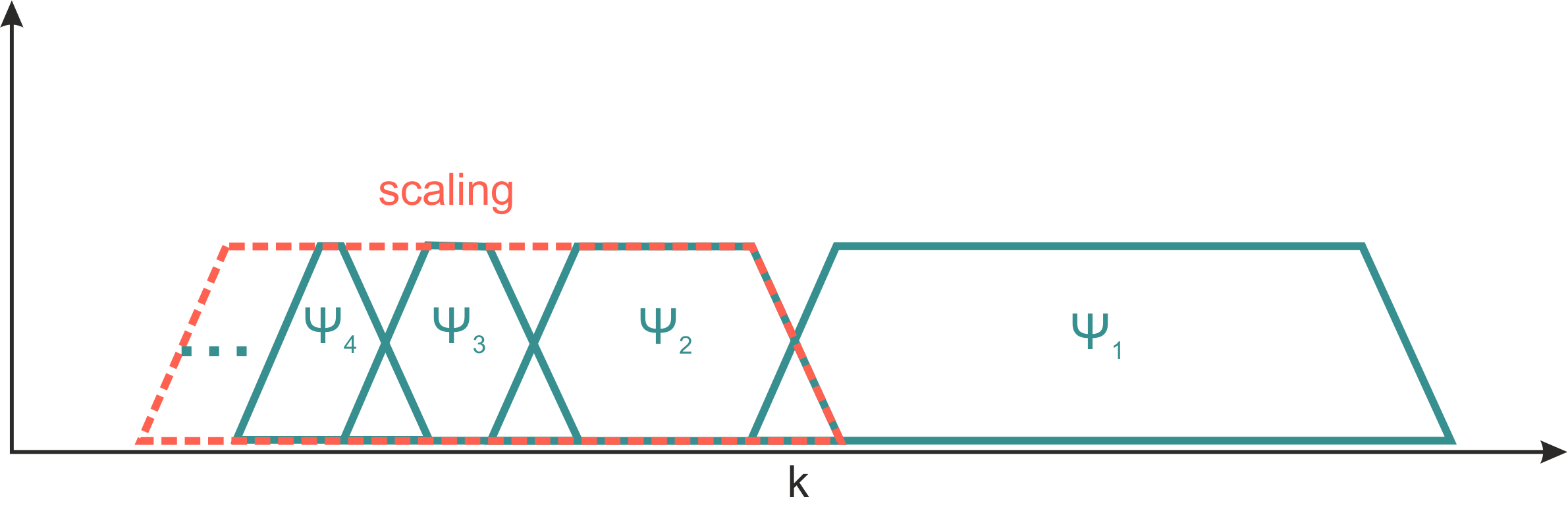
Discrete Wavelet Transform: Frequency enclosure is halved with each scaling step. The filterbank decomposition splits into wavelet (high-pass detail) and scaling (low-pass approximation) components up to a specified level.
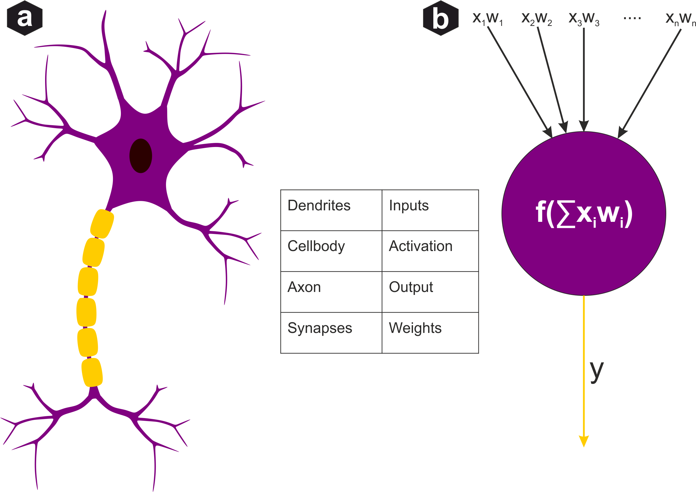
Biological neuron vs artificial perceptron: Biological neuron receives signals through dendrites, processes in soma, outputs via axon. Artificial perceptron weights inputs, sums them with bias, applies non-linear activation function.
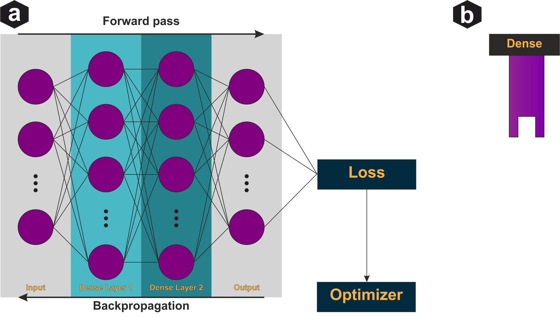
Dense (fully connected) layer: Each output is a weighted sum of all inputs plus bias, passed through activation. Trainable parameters are all weight connections. A feedforward network stacks dense layers with non-linear activations between them.
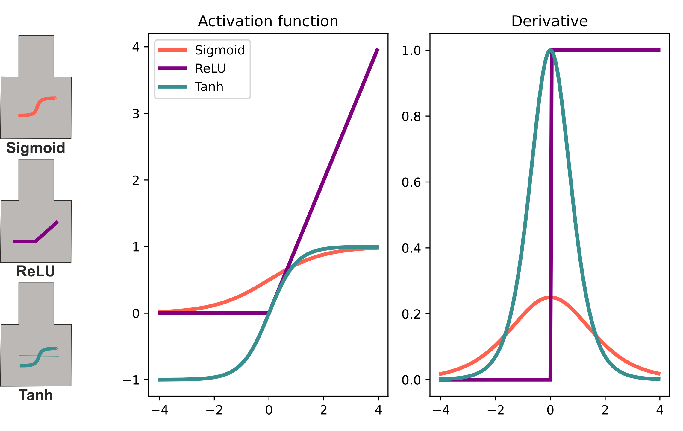
Activation functions and derivatives: Sigmoid, Tanh, and ReLU. Sigmoid and Tanh saturate for large positive/negative values, causing vanishing gradients during backpropagation. ReLU saturates only for negative values (dying ReLU problem).
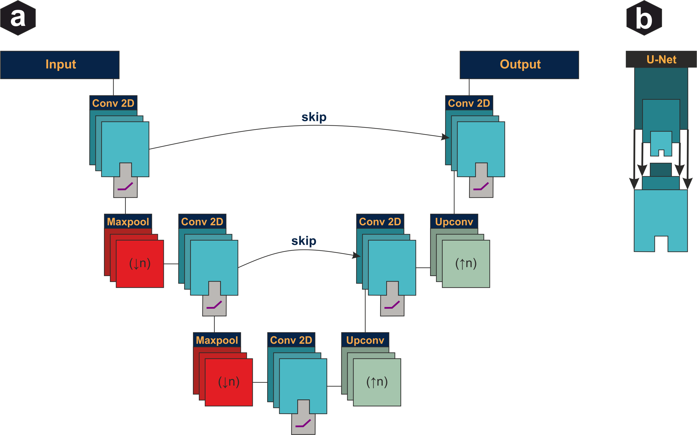
U-Net architecture: Encoder-decoder structure with skip connections. Contracting path (left) extracts hierarchical features through convolutions and pooling. Expanding path (right) reconstructs spatial information. Skip connections preserve fine details lost during downsampling.
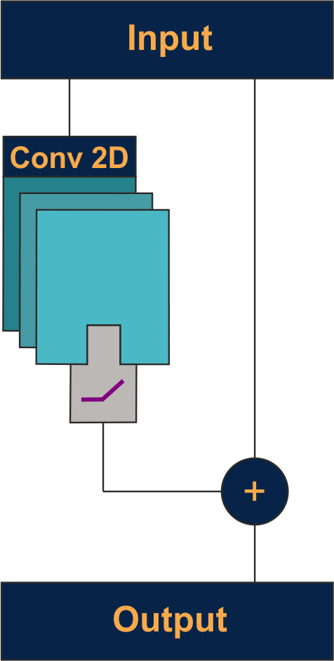
ResNet: Identity shortcuts skip every few layers, allowing gradients to flow directly through the network. This addresses vanishing gradients in very deep networks and enables training of 100+ layer architectures.
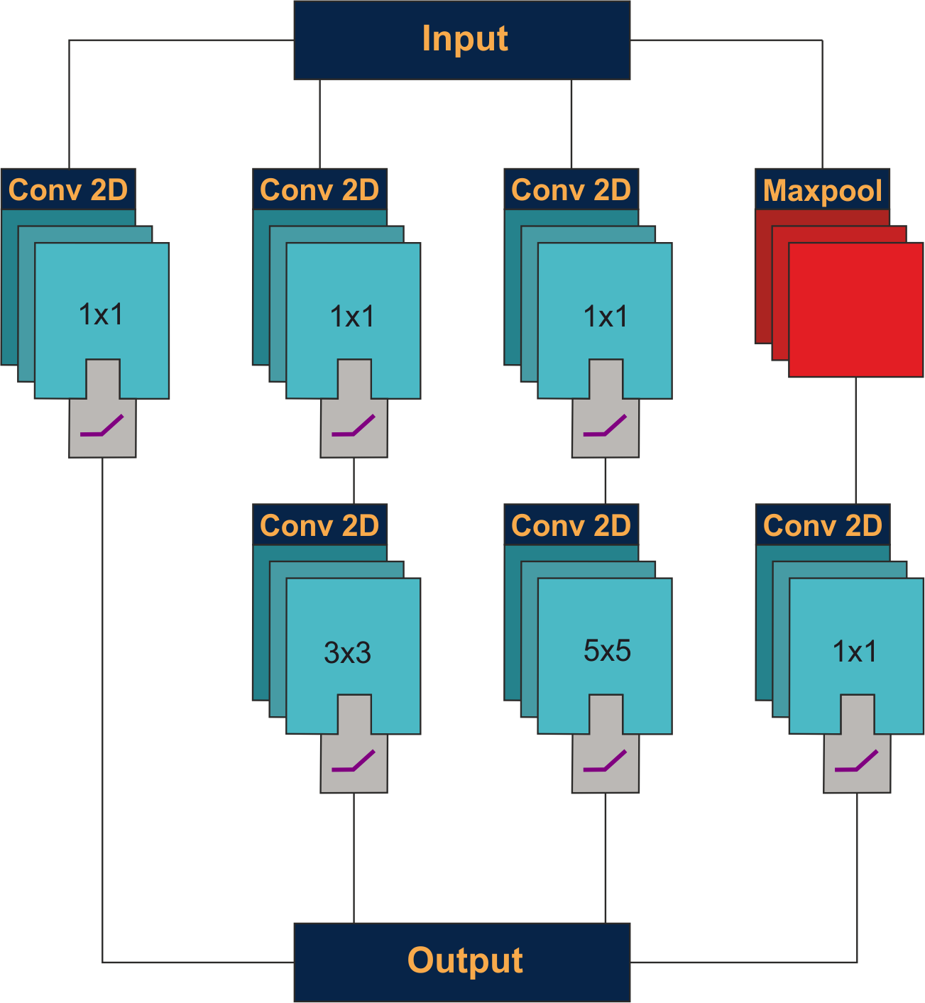
Inception V1 module: Parallel branches apply 1×1, 3×3, 5×5 convolutions and max-pooling simultaneously. Outputs are concatenated. 1×1 convolutions before larger kernels reduce computational cost by compressing channel dimensions.
Sections
Results & Applications
From theory to production software
Practical applications of the developed methods: LineProfiler for microtubule and synaptonemal complex evaluation, Automated Elastix for expansion factor determination, and ReCSAI achieving state-of-the-art precision for confocal dSTORM reconstruction.
Key Figures
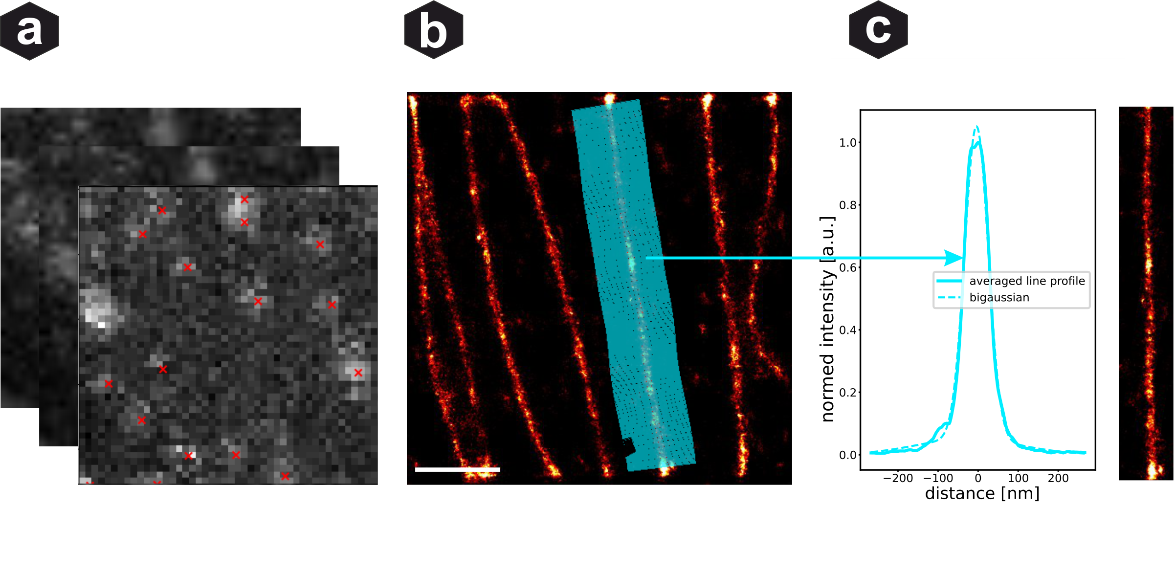
ReCSAI evaluation: (a) AI fitting of disrupted PSFs - red crosses mark estimated fluorophore locations. (b) Reconstructed super-resolution image with line profiles marked. (c) Averaged line profile with bi-Gaussian fit showing the resolved microtubule structure.
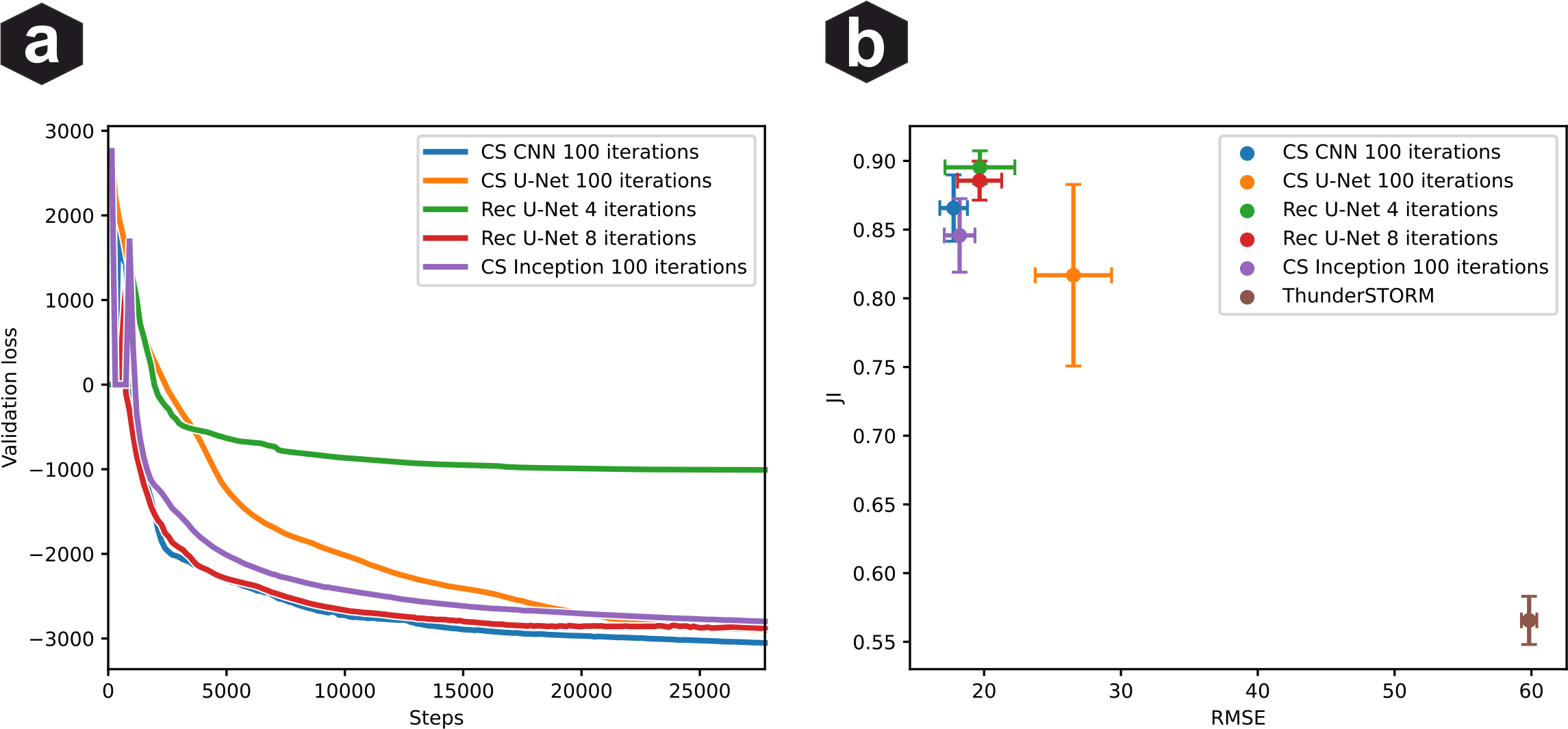
Network architecture comparison: (a) Validation loss vs training steps for different architectures. (b) Jaccard Index and RMSE metrics. ThunderSTORM fitting shown as baseline. Error bars show standard deviation over N=25 validation datasets.
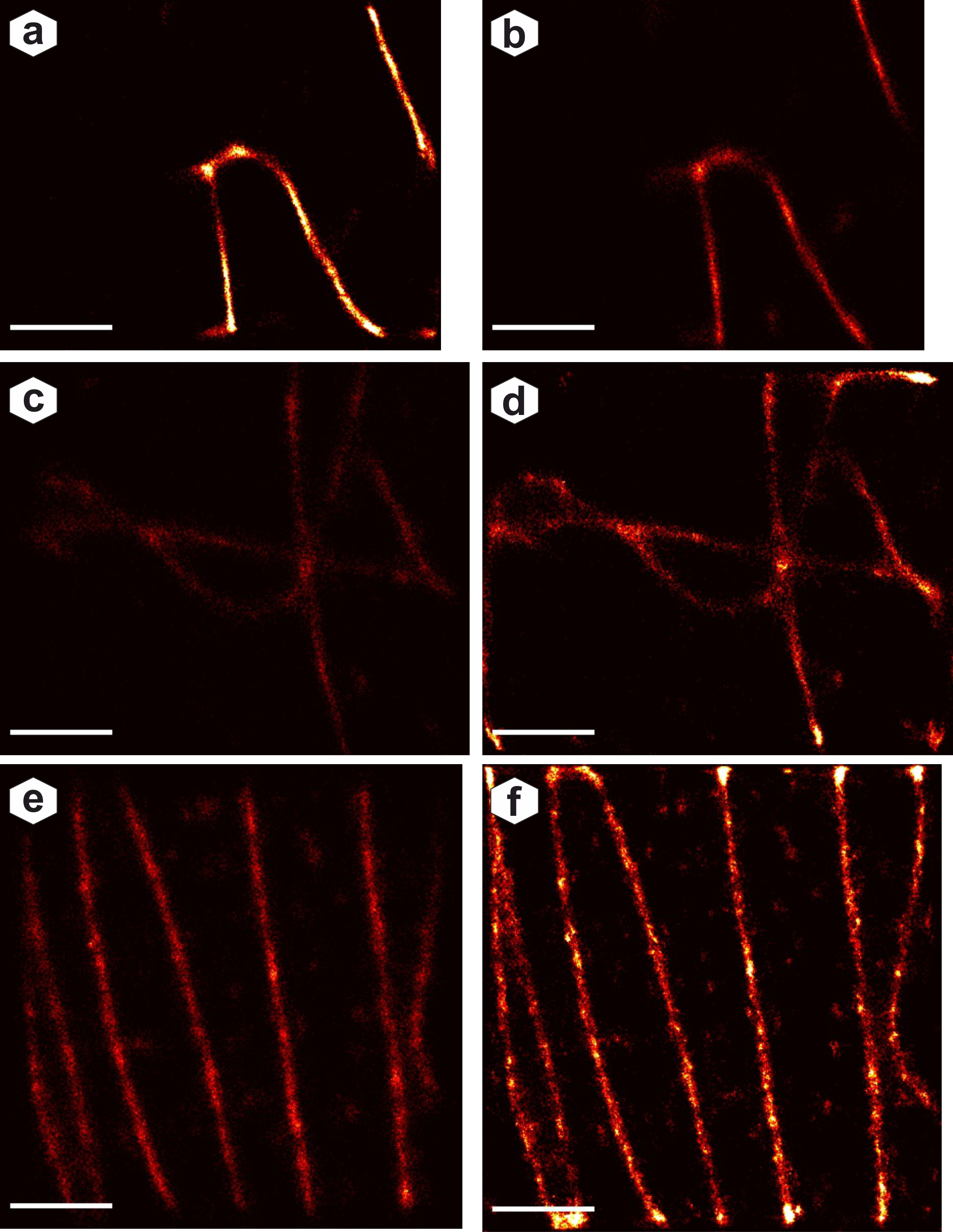
Reconstruction comparison: AI reconstruction (left) vs ThunderSTORM (right) for three test images. Fourier Ring Correlation coefficients quantify resolution - AI achieves higher FRC values indicating better reconstruction quality.
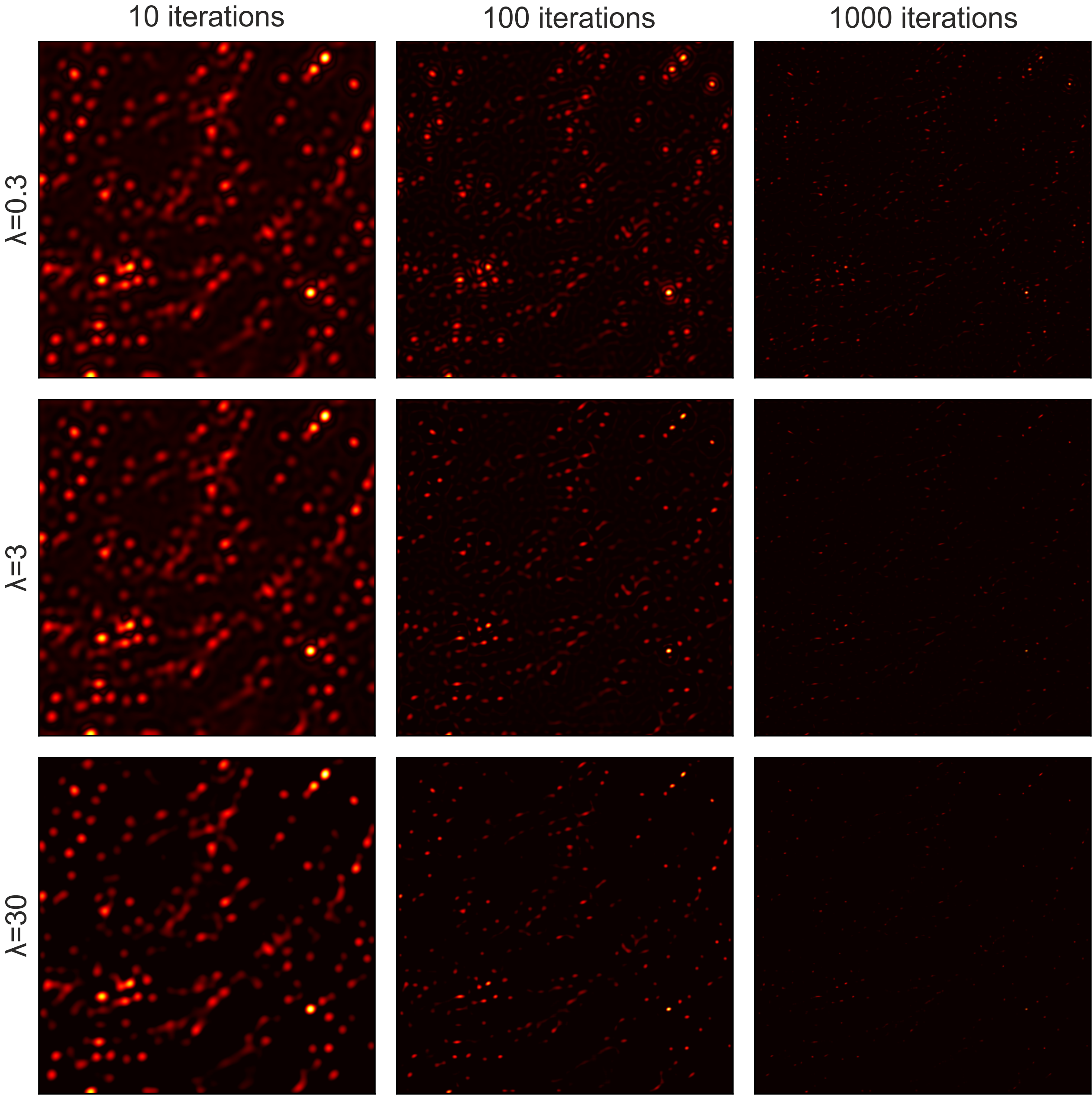
Compressed Sensing hyperparameters: Lower λ reduces noise but slows convergence. Higher λ speeds up reconstruction but risks losing weak emitters by classifying them as background. Trade-off must be optimized per dataset.
ReCSAI architecture: Algorithm unrolling integrates Compressed Sensing into the neural network. The model iteratively switches between feature and image space, receiving feedback on reconstruction quality at each iteration.
LineProfiler GUI: User-friendly interface for evaluating filamentous structures. Automated detection of line-shaped structures with sub-pixel accuracy for position and orientation determination.